English
 العربية
 Deutsch
 Français
PICTURE
The KL divergence is a way to measure how one probability distribution, let’s call it \( Q(x) \) differs from another probability distribution \( P(x) \).
import io
import soundfile as sf
import numpy as np
from transformers import AutoProcessor

# Load the Whisper processor (this contains both feature extractor and tokenizer)
processor = AutoProcessor.from_pretrained("openai/whisper-medium")

def bytes_to_array(audio_bytes, samplerate=16000):
    """
    Convert raw audio bytes to a numpy array.

    Args:
        audio_bytes (bytes): The raw audio data.
        samplerate (int): The sampling rate for the audio.

    Returns:
        tuple: A tuple containing the numpy array of audio data and the sampling rate.
    """
    audio_buffer = io.BytesIO(audio_bytes)
    data, sr = sf.read(audio_buffer, dtype="float32")
    return np.array(data), sr

def prepare_dataset(batch):
    """
    Process a single batch sample:
    - Extract audio features from the raw audio bytes.
    - Tokenize the transcript for the decoder.

    The processed sample will have:
      - "input_features": the extracted audio features.
      - "labels": tokenized transcript.
    """
    # Process the audio input: convert bytes to a numpy array and extract features
    audio, _ = bytes_to_array(batch["audio"]['bytes'])
    audio_inputs = processor.feature_extractor(audio, sampling_rate=16000, return_tensors="pt")
    batch["input_features"] = audio_inputs.input_features[0]

    # Tokenize the transcript (label) for the decoder
    labels = processor.tokenizer(batch["transcript"], return_tensors="pt", padding="longest")
    batch["labels"] = labels.input_ids[0]

    return batch

# Apply the tokenization function to the dataset while removing unnecessary columns
talkbank = talkbank.map(
    prepare_dataset,
    remove_columns=[
        'language_code', 'subset', 'full_language', 'switch_id', 'transcript_filename',
        'orig_file_start', 'orig_file_end', 'channel'
    ],
    num_proc=4
)
talkbank
DatasetDict({
    train: Dataset({
        features: ['audio', 'transcript', 'segment_id', 'audio_len_sec', 'input_features', 'labels'],
        num_rows: 1000
    })
    test: Dataset({
        features: ['audio', 'transcript', 'segment_id', 'audio_len_sec', 'input_features', 'labels'],
        num_rows: 1000
    })
})
import numpy as np
# Inspect the shape of the input features of sample index 42 from the test set
#print("Shape of input features:", np.asarray(talkbank["test"][42]["input_features"]).shape)

# Play the audio of sample index 42 (requires IPython.display)
import IPython.display as ipd

id = 500
sample, sr = bytes_to_array(talkbank["test"][id]["audio"]['bytes'])
transcript = talkbank['test']['transcript'][id]

print("Transcript:", transcript)
ipd.display(ipd.Audio(sample, rate=16000))
Transcript: oh my goodness .
talkbank['train']
Dataset({
    features: ['audio', 'transcript', 'segment_id', 'audio_len_sec', 'input_features', 'labels'],
    num_rows: 1000
})
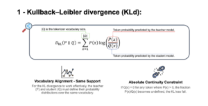
In the context of knowledge distillation for models, \( P(x) \) represents the token probabilities predicted by the teacher model, while \( Q(x) \) represents the token probabilities predicted by the student mode .
Why is it important?
The KL divergence helps the student model learn by comparing its predictions to the teacher’s predictions. It tells us how “close” the student’s predictions are to the teacher’s, and the goal during training is to make the KL divergence as small as possible.
How is it calculated?
Given the shared vocabulary |\( \Omega \)| , KL divergence is defined as:
\[
D_{KL}(P \parallel Q) = \sum_{x=1}^{|\Omega|} P(x) \log \left( \frac{P(x)}{Q(x)} \right)
\]
Here’s what this means:
-
\(P(x)\): The probability assigned by the teacher.
-
\(Q(x)\): The probability assigned to the same token the student.
-
The ratio \( \frac{P(x)}{Q(x)} \) “tell us how much” the student probability differs from student one for token x.
-
Finally we get \( P(x) \log \left( \frac{P(x)}{Q(x)} \right) \): with the purpose of multiplying by \( P(x) \) is to weight the difference between \( P(x) \) and \( Q(x) \) based on how important x is according to the teacher model.
The sum of these costs over all tokens in the vocabulary gives the KL divergence. If the student predicts exactly like the teacher (\( P(x) \) = \( Q(x) \) for all x), the KL divergence becomes 0, meaning perfect alignment.
Why vocabulary must be the same?
If the vocabularies differ, say that the student vocabulary is {dog, cat, sun} and the teacher one {dog, cat, moon}, then the probability for \( Q(moon) \) does not exist. In this case \( Q(moon) = 0 \) and \( \frac{P(x)}{Q(x)} \) becomes undefined (division by zero). This breaks the computation and makes the comparison inconsistent.
At Diabolocom, in partnership with CentraleSupélec and our PhD student Nicolas Boizard , we developed a new method called ULD Loss, based on Optimal Transport solutions rather than the classical Kullback-Leibler Divergence for knowledge distillation. For detailed information and improved results, you can access the paper here (accepted to TMLR ) but today, we will focus on understanding why the Wasserstein distance overcomes the requirement for identical vocabularies between the student and teacher models.
PICTURE
Overview:
The Wasserstein distance is another way to measure the difference between two probability distributions. It is also known as the Earth Mover’s Distance (EMD), and it provides a more geometrically intuitive measure of how much “work” is needed to transform one distribution into another.
How is it calculated?
The Wasserstein distance is defined as:
\[
W_p(P, Q) = \min_{T \in \Pi(P, Q)} \sum_{i=1}^{|\Omega_s|} \sum_{j=1}^{|\Omega_t|} T_{ij} C_{ij}^p
\]
Here’s what this means:
-
Pand \(Q\) are the probability distributions of the teacher and student, respectively.
-
\( T \in \Pi(P, Q) \) is the set of all couplings (joint distributions) between Pand \( Q \), meaning that each token in the teacher vocabulary is paired with a token in the student vocabulary.
-
\( C_{ij} \) is the transport cost, in our we can see it as the cost to transform \( Q(x) \) in \( P(x) \)
-
\(\displaystyle \min_{T \in \Pi(P, Q)} \sum_{i=1}^{|\Omega_s|} \sum_{j=1}^{|\Omega_t|} T_{ij} C_{ij}^{p}\) finally, meaning that we try to find the set of all couplings minimizing the cost to transform \( Q(x) \) into \( P(x) \).
Unlike KL divergence, the Wasserstein distance does not require that the vocabularies of the two models P (teacher) and Q (student) match. This is because we are comparing distributions in a more flexible, continuous manner. Each token from P can be mapped to any token in Q, regardless of whether the specific tokens appear in both vocabularies. However, similarly to the KL divergence, the Wasserstein distance value is minimal in both cases when (\( P(x) \) = \( Q(x) \) for all x. In this case, training the student model to reduce this value, forces the student model to reproduce the behavior of the teacher, or in other words, distills the teacher’s knowledge into the student’s model.
3 – Final thoughts
The ULD loss efficiently distills knowledge between models with different vocabularies (cf. our paper). This provides greater flexibility in selecting models for a teacher-student setup, particularly for models trained on different data distributions (different languages for example).